
Tips for functional MRI and resting state analysis
First take a quick look at your data.
library(ANTsR)
fn <- getANTsRData("KK")  # 4D image
img <- antsImageRead(fn, 4)
#' get the average to look at it in 3D
avg <- new("antsImage", dimension = 3, pixeltype = img@pixeltype)
antsMotionCorr(list(d = 3, a = img, o = avg))
#' look at the header to determine slices to display
ImageMath("4", "na", "PH", img)
par(mfrow = c(2, 1))
plotANTsImage(myantsimage = avg, slices = "12x33x3", axis = 3)
maskThresh <- 1e+05
mask <- getMask(avg, maskThresh, 1e+09, cleanup = TRUE)
# check if the mask is ok
plotANTsImage(myantsimage = avg, functional = list(mask), slices = "12x33x3",
    axis = 3, threshold = "0.5x1.5")
# The mask looks fine ( does not have to be perfect ) so we proceed.
The data looks ok so now convert the rsf image to a frequency filtered matrix.
This involves motion correction which, with default settings, can be time consuming (because we are being careful). Here, we speed things up by setting moreaccurate=FALSE (not recommended).
We also estimate a brain mask and nuisance pararmeters including global signal, physiological and motion confounds. See /Users/stnava/code/RLibs/ANTsR/help/filterfMRIforNetworkAnalysis .
fmat <- timeseries2matrix(img, mask)
myres <- filterfMRIforNetworkAnalysis(fmat, tr = 4, 0.01, 0.1, cbfnetwork = "BOLD",
    mask = mask)

ANTsR preprocessing, including frequency filtering, for fMRI
The stage above factored out what many consider to be the major signals in fMRI that are not due to natural resting-state fluctuations in brain activity.
A network analysis may now be performed on the results of the above processing. The key output is myres$filteredTimeSeries. Let”s look at sample voxels” time series using basic plotting.
library(ggplot2)
samplevox1 <- round(ncol(myres$filteredTimeSeries)/2)
samplevox2 <- round(ncol(myres$filteredTimeSeries)/3)
data <- data.frame(time = c(1:nrow(myres$filteredTimeSeries)) * 4, v1 = myres$filteredTimeSeries[,
    samplevox1], v2 = myres$filteredTimeSeries[, samplevox2])
p1 <- (ggplot(data, aes(x = time, y = v1)) + geom_line() + ggtitle("Time series @ voxel 1"))
p2 <- (ggplot(data, aes(x = time, y = v2)) + geom_line() + ggtitle("Time series @ voxel 2"))
multiplot(p1, p2, cols = 1)  # function stolen from the internet
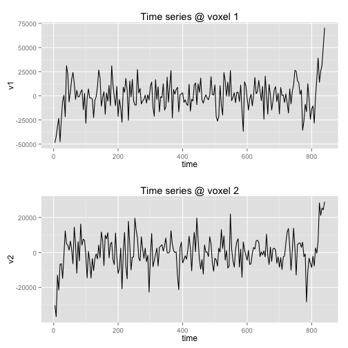
ANTsR sample voxels
That”s good — check a separate page for example network analyses. In brief, a network analysis will compute correlations between voxels such as these.
Let’s simulate a standard rsf network analysis by extracting some data-driven “ROIs” and show the resulting correlation matrix.
mysvd <- svd(myres$filteredTimeSeries)
# let's make the v eigenvectors sparse , otherwise they are totally
# uncorrelated
nevecs <- 10
vecs <- mysvd$v[, 1:nevecs]
thresh <- 0.005  # just an example
for (i in c(1:nevecs)) {
    vecs[, i] <- (vecs[, i] * (vecs[, i] > thresh))
    vecimg <- antsImageClone(myres$mask, "float")
    mask <- antsImageClone(myres$mask, "float")
    vecimg[(myres$mask > 0)] <- vecs[, i]
    ImageMath("3", vecimg, "ClusterThresholdVariate", vecimg, mask, "100")
    vecs[, i] <- vecimg[(myres$mask > 0)]
}
tobecorrelated <- (myres$filteredTimeSeries %*% vecs)
#' visualize the resulting correlations
image(cor(tobecorrelated))
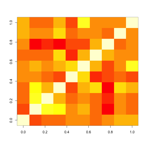
ANTsR rsfmri correlations from simple sparse svd
The correlation matrix is the most frequently used basis of rsf-MRI analysis.
Now you can reduce your fMRI data to relatively simple measurements of connectivity. Congratulations!
ToDo: add gray matter mask and anatomical labels.
## [1] "FAILURE: 17 vs refval 22"